NBAyesian Career Trajectories

Motivation

As part of our Bayesian Statistics book club, I wanted to demonstrate a use case of Bayesian techniques while familiarizing myself with some of the hierarchical modeling tools in python (read: PyMC). Since I had some experience with sabermetrics and R and wanted to do something slightly different, I settled on the following question.

How can one model NBA players’ career trajectories?

This question has much relevance for players, coaches, general managers, fans, and others. I’ll mostly follow the lead of Jim Albert’s excellent blog post on an analogous question for MLB players. Although there are many ways NBA players contribute to their teams’ success, we’ll narrow our scope and only use three pieces of information: who the player is, their age, and how many points they scored each season. First let’s grab the data and pare it down to the career stats of players who played last season and who have played at least three seasons.

Code

import numpy as np
import pandas as pd
import nba_api
from nba_api.stats.endpoints import leaguedashplayerstats
import matplotlib.pyplot as plt
import numpy as np
import plotly.express as px
import plotly.graph_objects as go
from time import sleep
from sklearn.preprocessing import PolynomialFeatures
from sklearn.linear_model import LinearRegression
import arviz as az
import seaborn as sns
import pymc as pm
import pytensor.tensor as pt


pd.set_option('display.max_columns', None)
pd.options.display.float_format = "{:,.2f}".format

Code

# Last 25 NBA seasons
start_year = 2000
end_year = 2025

seasons = [f"{y}-{str(y+1)[-2:]}" for y in range(start_year, end_year)]

Code

all_seasons_data = []

for season in seasons:
    print(f"Fetching {season}...")

    stats = leaguedashplayerstats.LeagueDashPlayerStats(
        season=season,
        season_type_all_star="Regular Season",
        per_mode_detailed="Totals"
    ).get_data_frames()[0]

    # Keep only what we need
    stats = stats[["PLAYER_ID", "PLAYER_NAME", "PTS", "AGE"]].copy()
    stats["AGE"] = stats['AGE'].astype(int)
    stats["SEASON_ID"] = season

    all_seasons_data.append(stats)

    sleep(0.6)  # VERY important to avoid rate limits

Code

df = pd.concat(all_seasons_data, ignore_index=True)

Code

season_counts = (
    df.groupby("PLAYER_ID")["SEASON_ID"]
    .nunique()
    .reset_index(name="SEASONS_PLAYED")
)

current_players = stats["PLAYER_ID"]      # players who played in '24-'25; "stats" is last year's data
eligible_players = season_counts[
    season_counts["SEASONS_PLAYED"] >= 3
]["PLAYER_ID"]

filtered_df = df[df["PLAYER_ID"].isin(eligible_players) & df["PLAYER_ID"].isin(current_players)]

Two Wrong Approaches

Ignoring who the players are, only using age & points

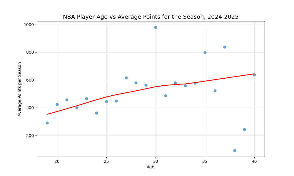
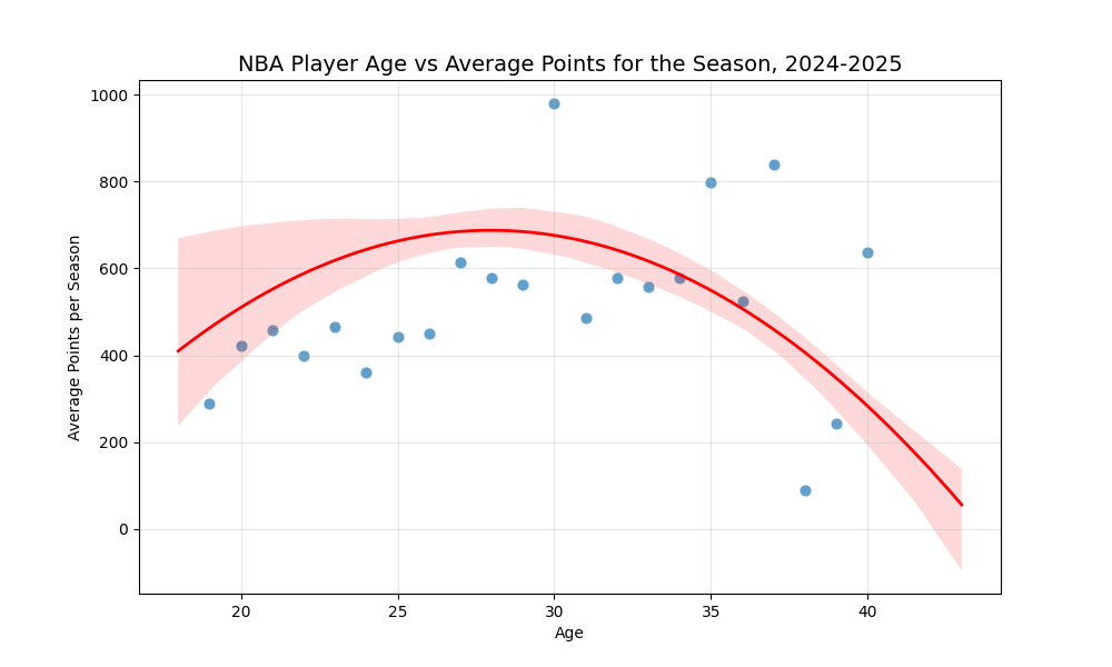
Let’s look at the average number of points scored by players during last season based on their age. The plot at the top of the page is fit with a LOESS model, and for simplicity, we can also fit a quadratic model:

\[Points_i = \beta_0 + \beta_1 Age_i + \beta_2 Age_i^2\]

Here’s the plot with a quadratic model.

Without much context, these might be surprising. The LOESS model shows that players continue to score more points on average as they age, and the quadratic model shows a decline, but it shows players continuing to score at a respectable rate, even in their late 30s. This is contrary to what we might expect from older players being less athletic. Why don’t teams fill their rosters with older players who are great at scoring? The issue with that logic is that there’s a survivorship bias. The following table, bar chart, and explanation break it down for us.

Age	Average Points	Number of Players
19	289.17	6
20	422.89	18
21	457.23	31
22	399.34	47
23	464.40	52
24	361.42	78
25	443.67	63
26	449.12	51
27	614.93	43
28	578.59	37
29	563.47	34
30	979.93	14
31	486.95	21
32	579.00	20
33	557.81	16
34	577.50	8
35	797.00	10
36	523.14	7
37	839.00	4
38	90.00	2
39	243.00	3
40	637.25	4

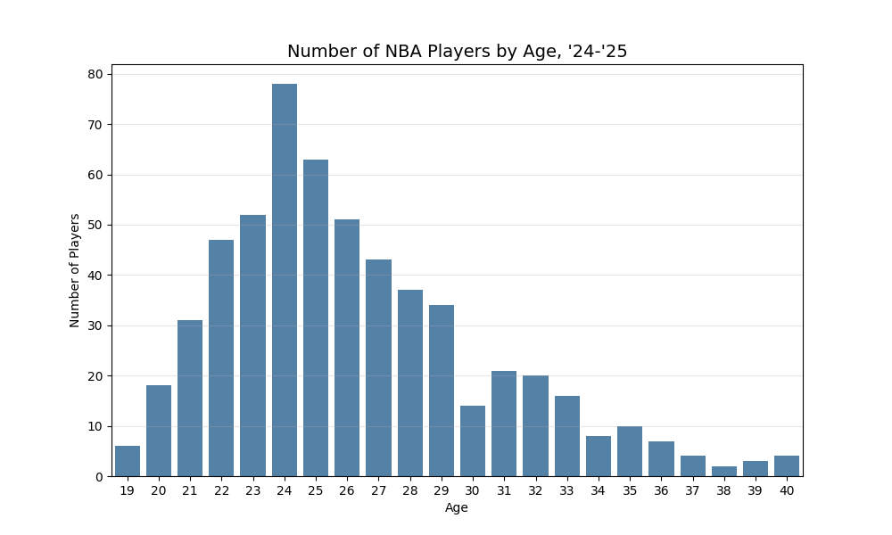
We can see there are a lot 20-something year-olds in the league, which is in tune with what we might’ve originally expected. The older ages have high scoring averages because the only players who are that age and are still in the league are stars who are past their peaks but are still good enough to contribute to their teams. Or to paraphrase what I told my sabermetrics class, “if we only looked at players with over 20 years of playing time, the results are pretty skewed since we’re only looking at LeBron James, who isn’t representitve of players.” Here are all the players who were 40 years old last season.

PLAYER_NAME	PTS	AGE
Chris Paul	723	40
LeBron James	1710	40
P.J. Tucker	9	40
Taj Gibson	107	40

Surely, if we looked at all 40-year-olds who have played in the NBA and forced them back into the league, the average scoring for 40-year-olds would be much smaller.

Individual models

So how can we try to account for this and model career trajectories? The other end of the spectrum would be to ignore similarities across players and to fit individual models for each player. A quadratic model might seem like a good first approximation, and it looks as follows:

\[Points_i = \beta_{0,i} + \beta_{1,i} Age_i + \beta_{2,i} Age_i^2 \]

However, even with a lightweight model, this would be overfitting. For example, here are quadratic fits to all players who received an MVP vote in the ’24-’25 season.

Code

def fit_player_quadratic(player_df):
    X = player_df[["AGE"]].values
    y = player_df["PTS"].values

    poly = PolynomialFeatures(degree=2, include_bias=False)
    X_poly = poly.fit_transform(X)

    model = LinearRegression()
    model.fit(X_poly, y)

    return pd.Series({
        "beta_0": model.intercept_,
        "beta_age": model.coef_[0],
        "beta_age2": model.coef_[1],
        "n_obs": len(player_df),
        "age_min": player_df["AGE"].min(),
        "age_max": player_df["AGE"].max()
    })

Code

player_models = (
    df
    .groupby(["PLAYER_ID", "PLAYER_NAME"])
    .apply(fit_player_quadratic)
    .reset_index()
)

Code

players_to_plot = [
    "Shai Gilgeous-Alexander",
    "Nikola Jokić",
    "Giannis Antetokounmpo",
    "Jayson Tatum",
    "Donovan Mitchell",
    "LeBron James",
    "Cade Cunningham",
    "Anthony Edwards",
    "Stephen Curry",
    "Jalen Brunson",
    "James Harden",
    "Evan Mobley"
]

Code

def make_color_map(player_names):
    palette = px.colors.qualitative.Set2
    return {
        player: palette[i % len(palette)]
        for i, player in enumerate(player_names)
    }

Code

def plot_players_with_quadratics(
    df,
    model_df,
    player_names,
    age_grid_size=100,
    max_age=40,
    y_clip=(0, 3000)
):
    fig = go.Figure()
    color_map = make_color_map(player_names)

    for player in player_names:
        df_p = df[df["PLAYER_NAME"] == player]
        model_p = model_df[model_df["PLAYER_NAME"] == player].iloc[0]
        color = color_map[player]

        age_min = df_p["AGE"].min()
        age_max_obs = df_p["AGE"].max()

        # Scatter: observed data
        fig.add_trace(
            go.Scatter(
                x=df_p["AGE"],
                y=df_p["PTS"],
                mode="markers",
                name=f"{player}",
                marker=dict(color=color, size=8),
                legendgroup=player,
                showlegend=True
            )
        )
        # Full age grid
        ages_full = np.linspace(age_min, max_age, age_grid_size)

        pts_full = (
            model_p["beta_0"]
            + model_p["beta_age"] * ages_full
            + model_p["beta_age2"] * ages_full**2
        )

        # Replace out-of-range values with None (line breaks)
        pts_plot = np.where(
            (pts_full >= y_clip[0]) & (pts_full <= y_clip[1]),
            pts_full,
            None
        )

        # Observed vs extrapolated masks
        obs_mask = ages_full <= age_max_obs

        fig.add_trace(
            go.Scatter(
                x=ages_full,
                y=np.where(obs_mask, pts_plot, None),
                mode="lines",
                name=f"{player} (fit)",
                line=dict(color=color, width=3),
                legendgroup=player,
                showlegend=False
            )
        )
        fig.add_trace(
            go.Scatter(
                x=ages_full,
                y=np.where(~obs_mask, pts_plot, None),
                mode="lines",
                name=f"{player} (projected)",
                line=dict(color=color, width=3, dash="dash"),
                legendgroup=player,
                showlegend=False
            )
)


    fig.update_layout(
        title="Player Scoring Trajectories with Quadratic Fits, MVP Vote Getters",
        xaxis_title="Age",
        yaxis_title="Total Points (Season)",
        template="plotly_white",
        hovermode="closest",
        yaxis=dict(range=list(y_clip))
    )

    return fig

Code

fig = plot_players_with_quadratics(
    df,
    player_models,
    players_to_plot
)

fig.show()

Though some of the quadratic curves fit the data well, some of them predict unrealistic trajectories. In particular, the parabolas for Shai Gilgeous-Alexander, Cade Cunningham, Donovan Mitchell, and Evan Mobley all open upwards, which doesn’t make sense since in reality, they’ll eventually start to decline. Also, as great as Jalen Brunson is, his extremely late peak here doesn't make sense. Our choice in a quadratic model can partially be blamed, but so can our choice of fitting a unique model for each individual. By fitting individual models, we’re missing out on relationships between the parameters of different players. Bayesian statistics can help us resolve this.

Multilevel model

Instead of fitting individual models, we can use a multilevel model. These types of models are good for data that can be grouped at multiple levels. In this case, each datapoint consists of a player, his age, and how many points he scored. Our first type of model ignored the relationships at the player level, though this is important; players perform at different levels, with different peaks and improvement/decline rates. The second type of model we fit ignored relationships across the players at different ages, and this information is useful because biology and experience lead to players having similarly shaped trajectories.

The Bayesian philosophy is as follows. We can again use the framework of the quadratic model

\[Points_i = \beta_{0,i} + \beta_{1,i} Age_i + \beta_{2,i} Age_i^2 \]

However, this time, we assume that the coefficients \(\beta_{0,i}\) come from a distribution, as do the \(\beta_{1,i}\) and \(\beta_{2,i}\). These assumptions impose a regularization on the coefficients and ensure that they don’t solely consider the individual player, but rather also overall scoring vs. age trends. The assumptions look like

\[\beta_{0,i} \sim N(\mu_0, \sigma_0^2)\] \[\beta_{1,i} \sim N(\mu_1, \sigma_1^2)\] \[\beta_{2,i} \sim N(\mu_2, \sigma_2^2)\]

We initialize the prior distributions and values of \(\mu\)s and \(\sigma\)s and then the model uses Bayes’ theorem to take the priors and data to compute the posterior distributions. Full disclosure: I got this code from ChatGPT. My first attempt had too many divergences and it suggested using the LKJ prior and a non-centered parametrization, and when I used the updated code it gave, it worked. Here’s how it explains each part. The short explanation is that the means \(\mu_0, \mu_1\), and \(\mu_2\) are population-level mean coefficients. We can use domain knowledge and intuition to initialize them in a way that makes sense, but ChatGPT just set them as 0 and I ran with it to try to get things to run. The values of \(\sigma\) are initialized as \(10, 5\), and \(5\), and I think we could probably loosen these (make \(\sigma\)s larger) if we’re worried about underfitting and tighten them (reduce initialized \(\sigma\)s) if we think we may be overfitting. But I digress, and here’s the code to do this.

Code

player_idx, player_ids = pd.factorize(filtered_df["PLAYER_ID"])
filtered_df["PLAYER_ID"] = player_idx

age = filtered_df["AGE"].values
points = filtered_df["PTS"].values
player_idx = filtered_df["PLAYER_ID"].values

n_players = filtered_df["PLAYER_ID"].nunique()

Code

age_c = age - age.mean()
age_c2 = age_c ** 2

Code

with pm.Model() as model:

    # ---- Population means ----
    mu_beta = pm.Normal(
        "mu_beta",
        mu=[0.0, 0.0, 0.0],
        sigma=[10.0, 5.0, 5.0],
        shape=3
    )

    # ---- Covariance of random effects ----
    chol, corr, sigmas = pm.LKJCholeskyCov(
        "chol",
        n=3,
        eta=2.0,
        sd_dist=pm.Exponential.dist(1.0),
        compute_corr=True
    )

    # ---- Non-centered random effects ----
    z = pm.Normal(
        "z",
        mu=0,
        sigma=1,
        shape=(n_players, 3)
    )

    beta = pm.Deterministic(
        "beta",
        mu_beta + pt.dot(z, chol.T)
    )

    beta0 = beta[:, 0]
    beta1 = beta[:, 1]
    beta2 = beta[:, 2]

    # ---- Linear predictor ----
    mu = (
        beta0[player_idx]
        + beta1[player_idx] * age_c
        + beta2[player_idx] * age_c**2
    )

    # ---- Observation noise ----
    sigma = pm.Exponential("sigma", 1.0)

    # ---- Likelihood ----
    points_obs = pm.Normal(
        "points_obs",
        mu=mu,
        sigma=sigma,
        observed=points
    )

    trace = pm.sample(
        2000,
        tune=2000,
        target_accept=0.9,
        chains=4
    )

We immediately see that all the trajectories are now downward opening, which matches what we’d expect from what we know about athletes’ careers. I think this might be overfitting a little bit because many of the players’ curves decline rather steeply. This analysis included all players who played in the ’24-’25 season, and we’re comparing so it includes hundreds of players who won’t have as long of careers or high of peaks as the MVP candidates we’re looking at here. One way we can assuage this overfitting is by relaxing our priors, increasing the hyperparameters for the \(\sigma\).

Comparing the three models

One way we can compare the three models shown above is by seeing how well they predict future values. Instead of waiting for the current season (‘25-’26) to end, we can fit the model on the players’ data up to but not including ’24-’25, then see how well the model does in predicting the ’24-’25 scoring totals. We’ll look at both the mean squared error and the mean absolute error as our metrics to compare the performance.

I’ll show the results first and then the code for it after.

Results

	MSE	MAE
Age-only	434,242.99	475.02
Per-player	551,429.81	568.89
Hierarchical	116,174.63	267.22

We see that under both metrics, the hierarchical model vastly outperforms the other two. The way to interpret the errors is that on average, our hierarchical model prediction for the ’24-’25 season is about 267 points away from the true value and the squared error is 116 thousand squared points.

Prepping the data

Code

df2 = filtered_df.copy()

# Extract ending year (e.g. "2024-25" → 20252
2df["season_end"]=2 2df["SEASON_ID"].str.split("-").str[1].astype(int)

Code

train_df = df2[df2["season_end"] <= 24]
test_df  = df2[df2["season_end"] == 25]

Code

age_mean = train_df["AGE"].mean()

train_df["age_c"] = train_df["AGE"] - age_mean
test_df["age_c"]  = test_df["AGE"] - age_mean

Code

age_train = train_df["age_c"].values
points_train = train_df["PTS"].values

age_test = test_df["age_c"].values
points_test = test_df["PTS"].values

Code

# Unique players in training set
player_ids = train_df["PLAYER_ID"].unique()
n_players = len(player_ids)

player_id_to_idx = {
    pid: i for i, pid in enumerate(player_ids)
}

train_df["player_idx"] = train_df["PLAYER_ID"].map(player_id_to_idx)

Code

test_df = test_df[test_df["PLAYER_ID"].isin(player_ids)].copy()
test_df["player_idx"] = test_df["PLAYER_ID"].map(player_id_to_idx)

Code

player_idx_train = train_df["player_idx"].values
player_idx_test  = test_df["player_idx"].values

age_train = train_df["age_c"].values
points_train = train_df["PTS"].values

age_test = test_df["age_c"].values
points_test = test_df["PTS"].values

Code

test_df["player_idx"] = test_df["player_idx"].fillna(-1).astype(int)

Age-only model

Code

with pm.Model() as age_only_model:

    # ---- Priors ----
    beta0 = pm.Normal("beta0", mu=0.0, sigma=10.0)
    beta1 = pm.Normal("beta1", mu=0.0, sigma=5.0)
    beta2 = pm.Normal("beta2", mu=0.0, sigma=5.0)

    sigma = pm.Exponential("sigma", 1.0)

    # ---- Linear predictor ----
    mu = beta0 + beta1 * age_train + beta2 * age_train**2

    # ---- Likelihood ----
    points_obs = pm.Normal(
        "points_obs",
        mu=mu,
        sigma=sigma,
        observed=points_train
    )

    # ---- Sampling ----
    trace_age_only = pm.sample(
        2000,
        tune=2000,
        chains=4,
        target_accept=0.9,
        random_seed=42
    )

Code

posterior = trace_age_only.posterior

beta0_draws = posterior["beta0"].values.reshape(-1)
beta1_draws = posterior["beta1"].values.reshape(-1)
beta2_draws = posterior["beta2"].values.reshape(-1)

Code

mu_test_draws = (
    beta0_draws[:, None]
    + beta1_draws[:, None] * age_test[None, :]
    + beta2_draws[:, None] * age_test[None, :]**2
)

Code

mse_draws = np.mean((points_test[None, :] - mu_test_draws)**2, axis=1)
mse_age_only = mse_draws.mean()

mae_draws = np.mean(abs(points_test[None, :] - mu_test_draws), axis=1)
mae_age_only = mae_draws.mean()

Individual Models

Code

with pm.Model() as per_player_model:

    # ---- Player-specific coefficients (independent priors) ----
    beta0 = pm.Normal(
        "beta0",
        mu=0.0,
        sigma=10.0,
        shape=n_players
    )

    beta1 = pm.Normal(
        "beta1",
        mu=0.0,
        sigma=5.0,
        shape=n_players
    )

    beta2 = pm.Normal(
        "beta2",
        mu=0.0,
        sigma=5.0,
        shape=n_players
    )

    # ---- Observation noise ----
    sigma = pm.Exponential("sigma", 1.0)

    # ---- Linear predictor ----
    mu = (
        beta0[player_idx_train]
        + beta1[player_idx_train] * age_train
        + beta2[player_idx_train] * age_train**2
    )

    # ---- Likelihood ----
    points_obs = pm.Normal(
        "points_obs",
        mu=mu,
        sigma=sigma,
        observed=points_train
    )

    # ---- Sampling ----
    trace_per_player = pm.sample(
        2000,
        tune=2000,
        chains=4,
        target_accept=0.9,
        random_seed=42
    )

Code

posterior = trace_per_player.posterior

beta0_draws = posterior["beta0"].values.reshape(-1, n_players)
beta1_draws = posterior["beta1"].values.reshape(-1, n_players)
beta2_draws = posterior["beta2"].values.reshape(-1, n_players)

Code

mu_test_draws = (
    beta0_draws[:, player_idx_test]
    + beta1_draws[:, player_idx_test] * age_test
    + beta2_draws[:, player_idx_test] * age_test**2
)

Code

mse_draws = np.mean((points_test[None, :] - mu_test_draws)**2, axis=1)

mae_draws = np.mean(abs((points_test[None, :] - mu_test_draws)), axis=1)

mse_per_player = mse_draws.mean()
mae_per_player = mae_draws.mean()

Hierarchical Model

Code

with pm.Model() as hierarchical_model:

    # ---- Population means ----
    mu_beta = pm.Normal(
        "mu_beta",
        mu=[0.0, 0.0, 0.0],
        sigma=[10.0, 5.0, 5.0],
        shape=3
    )

    # ---- Covariance of random effects ----
    chol, corr, sigmas = pm.LKJCholeskyCov(
        "chol",
        n=3,
        eta=2.0,
        sd_dist=pm.Exponential.dist(1.0),
        compute_corr=True
    )

    # ---- Non-centered random effects ----
    z = pm.Normal(
        "z",
        mu=0.0,
        sigma=1.0,
        shape=(n_players, 3)
    )

    beta = pm.Deterministic(
        "beta",
        mu_beta + pt.dot(z, chol.T)
    )

    beta0 = beta[:, 0]
    beta1 = beta[:, 1]
    beta2 = beta[:, 2]

    # ---- Linear predictor (TRAIN ONLY) ----
    mu = (
        beta0[player_idx_train]
        + beta1[player_idx_train] * age_train
        + beta2[player_idx_train] * age_train**2
    )

    # ---- Observation noise ----
    sigma = pm.Exponential("sigma", 1.0)

    # ---- Likelihood ----
    pm.Normal(
        "points_obs",
        mu=mu,
        sigma=sigma,
        observed=points_train
    )

    # ---- Sampling ----
    trace_hier = pm.sample(
        2000,
        tune=2000,
        chains=4,
        target_accept=0.9,
        random_seed=42
    )

Code

posterior = trace_hier.posterior

beta_draws = posterior["beta"].values.reshape(-1, n_players, 3)
mu_beta_draws = posterior["mu_beta"].values.reshape(-1, 3)

n_draws = beta_draws.shape[0]
n_test = len(test_df)

mu_test_draws = np.zeros((n_draws, n_test))

for j in range(n_test):
    idx = player_idx_test[j]
    age = age_test[j]

    if idx == -1:
        b0, b1, b2 = mu_beta_draws.T
    else:
        b0 = beta_draws[:, idx, 0]
        b1 = beta_draws[:, idx, 1]
        b2 = beta_draws[:, idx, 2]

    mu_test_draws[:, j] = b0 + b1 * age + b2 * age**2

Code

mse_draws = np.mean((points_test[None, :] - mu_test_draws)**2, axis=1)
mae_draws = np.mean(abs((points_test[None, :] - mu_test_draws)), axis=1)

mse_hierarchical = mse_draws.mean()
mae_hierarchical = mae_draws.mean()

Further approaches and questions

We could go much deeper in several directions:

We could allow for a more flexible model than simply a quadratic one. FiveThirtyEight’s CARMELO system uses local regression and likely outperforms what we’ve done here.
We can further evaluate performance by looking at plots of the residuals, especially looking at residuals vs. age to see if there are major issues.
We can fine-tune the initialized hyperparameters using cross-validation.
This data included only players who played last season, and we can broaden the analysis to include players who have already retired. Presumably, some players will retire this season, so I don’t think our approach will bias things in one direction or another too much.
More advanced models could be built off of these ideas and incorporate additional features such as height, weight, position, usage rate, etc.
From what I gathered from McElreath’s book, the \(\mu\)s and the \(\sigma\)s would themselves come from distributions, and we’d select hyperparameters for those. I don’t fully see where that’s happening in the code, or if it’s happening at all. Is that just something that’s part of the theory but not explicit in practice due to the math working out really nicely with conjugate priors? If you have additional insight, please reach out!