How do we compare a movie with a single 5-star rating to one with many 4 and 5 ratings?
Say we want to take user ratings of movies and rank them. A simple approach would be to just look at the average rating of each movie, but that doesn’t feel right.. different movies have different amounts of ratings, and we don’t want small samples to skew our estimate of the ‘’true’’ rating that would arise if the whole population rated that movie. Smoothed (a.k.a. dampened) average ratings is one approach to handle this and is an example of a non-personalzed recommendation system. Let’s start by looking at the highest rated movies from the MovieLens dataset on Kaggle.
Code
# import the data# ratings doesn't include movie names so merge with ids to get namesratings = pd.read_csv("archive/rating.csv", parse_dates=['timestamp'])ids = pd.read_csv("archive/movie.csv")ratings = pd.merge(ratings, ids, on='movieId', how='left')# Find each movie's mean ratingavg_ratings = ratings.groupby(['movieId', 'title'])['rating'].agg( avg_rating='mean', rating_count='count')avg_ratings.sort_values(by ='avg_rating', ascending=False, inplace =True)avg_ratings.head()
movieId
Title
Mean Rating
Number of Ratings
117314
Neurons to Nirvana (2013)
5.0
1
117418
Victor and the Secret of Crocodile Mansion (2012)
5.0
1
117061
The Green (2011)
5.0
1
109571
Into the Middle of Nowhere (2010)
5.0
1
109715
Inquire Within (2012)
5.0
1
Not quite the blockbusters or classics we were expecting.. We’ll soon see that there are a bunch of movies that had just one rating with an average of 5 stars. We could filter the data to only include movies whose number of ratings is over a certain threshold \(m\), as this table does with \(m = 50\).
movieId
Title
Mean Rating
Number of Ratings
318
Shawshank Redemption, The (1994)
4.447
63366
858
Godfather, The (1972)
4.365
41355
50
Usual Suspects, The (1995)
4.334
47006
527
Schindler's List (1993)
4.310
50054
1221
Godfather: Part II, The (1974)
4.276
27398
2019
Seven Samurai (Shichinin no samurai) (1954)
4.274
11611
904
Rear Window (1954)
4.271
17449
7502
Band of Brothers (2001)
4.263
4305
912
Casablanca (1942)
4.258
24349
922
Sunset Blvd. (a.k.a. Sunset Boulevard) (1950)
4.257
6525
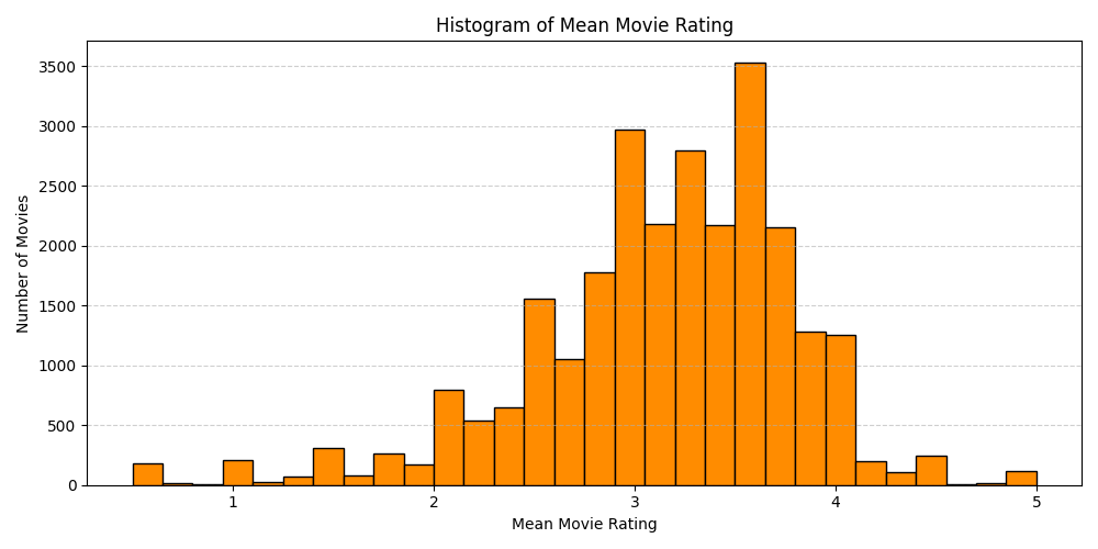
However, this is a little crude for a few reasons. It's tricky to pick a threshold \(m\) that is fair; lower values of \(m\) will allow movies with small sample sizes to pass, while higher values don't consider movies with \(m-1\) ratings, even if they're all 5-stars. By smoothing the means, we can balance these two competing stakes. A little bit of Exploratory Data Analysis to start.
Code
# Plot histogramplt.figure(figsize=(10, 5))plt.hist(avg_ratings['avg_rating'], bins=30, color='darkorange', edgecolor='black')plt.xlabel('Mean Movie Rating')plt.ylabel('Number of Movies')plt.title('Histogram of Mean Movie Rating')plt.grid(axis='y', linestyle='--', alpha=0.6)plt.tight_layout()plt.show()
Now let’s check out what the users are like. We see right away that there are users with dozens of ratings that rated all of their movies as 5-stars. The distribution of mean user ratings gives us a sense of how people tend to rate movies.
Code
# Find each user's mean ratinguser_avg_ratings = ratings.groupby('userId')['rating'].agg( user_avg_rating='mean', rating_count='count')user_avg_ratings.sort_values(by ='user_avg_rating', ascending=False, inplace =True)user_avg_ratings.head()
user_avg_rating
rating_count
5.000
20
5.000
35
4.949
39
4.893
56
4.827
52
Code
# Scatterplotplt.scatter(avg_ratings['avg_rating'], avg_ratings['rating_count'], s=5)plt.xlabel('Mean Movie Rating')plt.ylabel('Number of Ratings')plt.title('Scatterplot of Mean Movie Rating vs. Number of Ratings')plt.grid(True)plt.show()
This previous plot shows that there are a lot of movies with high means (even some 5.0s) that have few ratings. We may not want to necessarily recommend those movies to everyone, but the simplest recommender (that solely looks at mean movie rating) would recommend those.
Average Rating
This system simply takes the movies with the highest mean ratings and recommends them to everyone.
We’ve computed each movie’s mean rating and sorted by that mean rating, so the top movies according to this (admittedly poor) recommendation system would be those with the highest means, regardless of how many ratings there are.
There would be a 113-way tie for first place.. and the most ratings that any of those perfectly rated films has is 2.
Smoothed (dampened) average rating
The idea here is that instead of taking the rating to be the mean over the \(N_j\) ratings of movie \(j\), (i.e. \(r_j = \sum_i X_i/N_j\)), we can look at something like
Here, \(\mu_0\) and \(\lambda\) are hyperparameters. I’ll just take \(\mu_0\) to be the mean of all the ratings and \(\lambda = 1\) to start. This system gives unrated movies the mean rating \(\mu_0\) and as a movie gets more ratings, this rating converges towards its “true mean rating”, i.e. its rating across the whole population.
Code
# Step 1: Compute the global meanmu_0 = ratings['rating'].mean()damp_factor =1# Step 2: Group and compute sum and countdampened_avg_ratings = ratings.groupby(['movieId', 'title'])['rating'].agg( sum_rating='sum', rating_count='count').reset_index()# Step 3: Compute dampened meandampened_avg_ratings['dampened_mean'] = (dampened_avg_ratings['sum_rating'] + damp_factor*mu_0) / (dampened_avg_ratings['rating_count'] + damp_factor)
movieId
Title
Ratings Sum
Number of Ratings
Dampened Mean
108527
Catastroika (2012)
10.0
2
4.509
103871
Consuming Kids: The Commercialization of Childhood (2008)
10.0
2
4.509
98275
Octopus, The (Le poulpe) (1998)
14.5
3
4.506
318
Shawshank Redemption, The (1994)
281788.0
63366
4.447
113315
Zero Motivation (Efes beyahasei enosh) (2014)
49.5
11
4.419
Okay, that fourth spot being held by a critically-acclaimed movie is encouraging. We see the other spots are still held by movies with few ratings, and we can tweak the hyperparameter \(\lambda\) to further dampen the means. Here’s what the top 10 lists look like for various \(\lambda\).
Select a Dampening Factor (0–5):
Title
Dampened Mean
Ratings Sum
Number of Ratings
Neurons to Nirvana (2013)
5.0
5.0
1
Victor and the Secret of Crocodile Mansion (2012)
5.0
5.0
1
The Green (2011)
5.0
5.0
1
Into the Middle of Nowhere (2010)
5.0
5.0
1
Inquire Within (2012)
5.0
5.0
1
Freeheld (2007)
5.0
5.0
1
Who Killed Vincent Chin? (1987)
5.0
5.0
1
Marihuana (1936)
5.0
5.0
1
The Encounter (2010)
5.0
5.0
1
Foster Brothers, The (Süt kardesler) (1976)
5.0
5.0
1
Title
Dampened Mean
Ratings Sum
Number of Ratings
Catastroika (2012)
4.509
10.0
2
Consuming Kids: The Commercialization of Childhood (2008)
4.509
10.0
2
Octopus, The (Le poulpe) (1998)
4.506
14.5
3
Shawshank Redemption, The (1994)
4.447
281788.0
63366
Zero Motivation (Efes beyahasei enosh) (2014)
4.419
49.5
11
Echoes of the Rainbow (Sui yuet san tau) (2010)
4.381
14.0
3
Plastic Bag (2009)
4.381
14.0
3
Hellhounds on My Trail (1999)
4.381
14.0
3
Deewaar (1975)
4.381
14.0
3
All Passion Spent (1986)
4.381
14.0
3
Title
Dampened Mean
Ratings Sum
Number of Ratings
Shawshank Redemption, The (1994)
4.447
281788.0
63366
Godfather, The (1972)
4.365
180503.5
41355
Zero Motivation (Efes beyahasei enosh) (2014)
4.350
49.5
11
Usual Suspects, The (1995)
4.334
203741.5
47006
Octopus, The (Le poulpe) (1998)
4.310
14.5
3
Schindler's List (1993)
4.310
215741.5
50054
Godfather: Part II, The (1974)
4.276
117144.0
27398
Seven Samurai (Shichinin no samurai) (1954)
4.274
49627.5
11611
Rear Window (1954)
4.271
74530.5
17449
Band of Brothers (2001)
4.263
18353.0
4305
Title
Dampened Mean
Ratings Sum
Number of Ratings
Shawshank Redemption, The (1994)
4.447
281788.0
63366
Godfather, The (1972)
4.365
180503.5
41355
Usual Suspects, The (1995)
4.334
203741.5
47006
Schindler's List (1993)
4.310
215741.5
50054
Zero Motivation (Efes beyahasei enosh) (2014)
4.291
49.5
11
Godfather: Part II, The (1974)
4.276
117144.0
27398
Seven Samurai (Shichinin no samurai) (1954)
4.274
49627.5
11611
Rear Window (1954)
4.271
74530.5
17449
Band of Brothers (2001)
4.263
18353.0
4305
Casablanca (1942)
4.258
103686.0
24349
Title
Dampened Mean
Ratings Sum
Number of Ratings
Shawshank Redemption, The (1994)
4.447
281788.0
63366
Godfather, The (1972)
4.365
180503.5
41355
Usual Suspects, The (1995)
4.334
203741.5
47006
Schindler's List (1993)
4.310
215741.5
50054
Godfather: Part II, The (1974)
4.276
117144.0
27398
Seven Samurai (Shichinin no samurai) (1954)
4.274
49627.5
11611
Rear Window (1954)
4.271
74530.5
17449
Band of Brothers (2001)
4.262
18353.0
4305
Casablanca (1942)
4.258
103686.0
24349
Sunset Blvd. (a.k.a. Sunset Boulevard) (1950)
4.256
27776.5
6525
It turns out that the top 10 list doesn’t change as we increase \(\lambda\) from 5 to 10.
Finally, here’s a visualization that has both the original (undampened) rating (blue) and the dampened rating (orange) with \(\lambda = 5\), as well as the difference in the ratings (gray line). The visualization is only for a sample of 50 movies so it doesn’t get too cluttered. You can see that the movies with fewer ratings are pulled more towards the overall mean, and those with more ratings have budged less. There’s probably a good physics interpretation of what’s going on here.. perhaps computing the center of mass of a plank with a weight on it where the plank’s mass depends on \(\lambda\) and the weight on top of it has a mass that depends on the number of ratings and is placed according to the movie’s average rating. I don’t know enough physics to truly formalize this connection..
Further approaches and questions
Stay tuned for future posts on other recommender systems where I’ll answer questions such as
How does one select the hyperparameter \(\lambda\)?